LESSON 4 – Intervals and segments

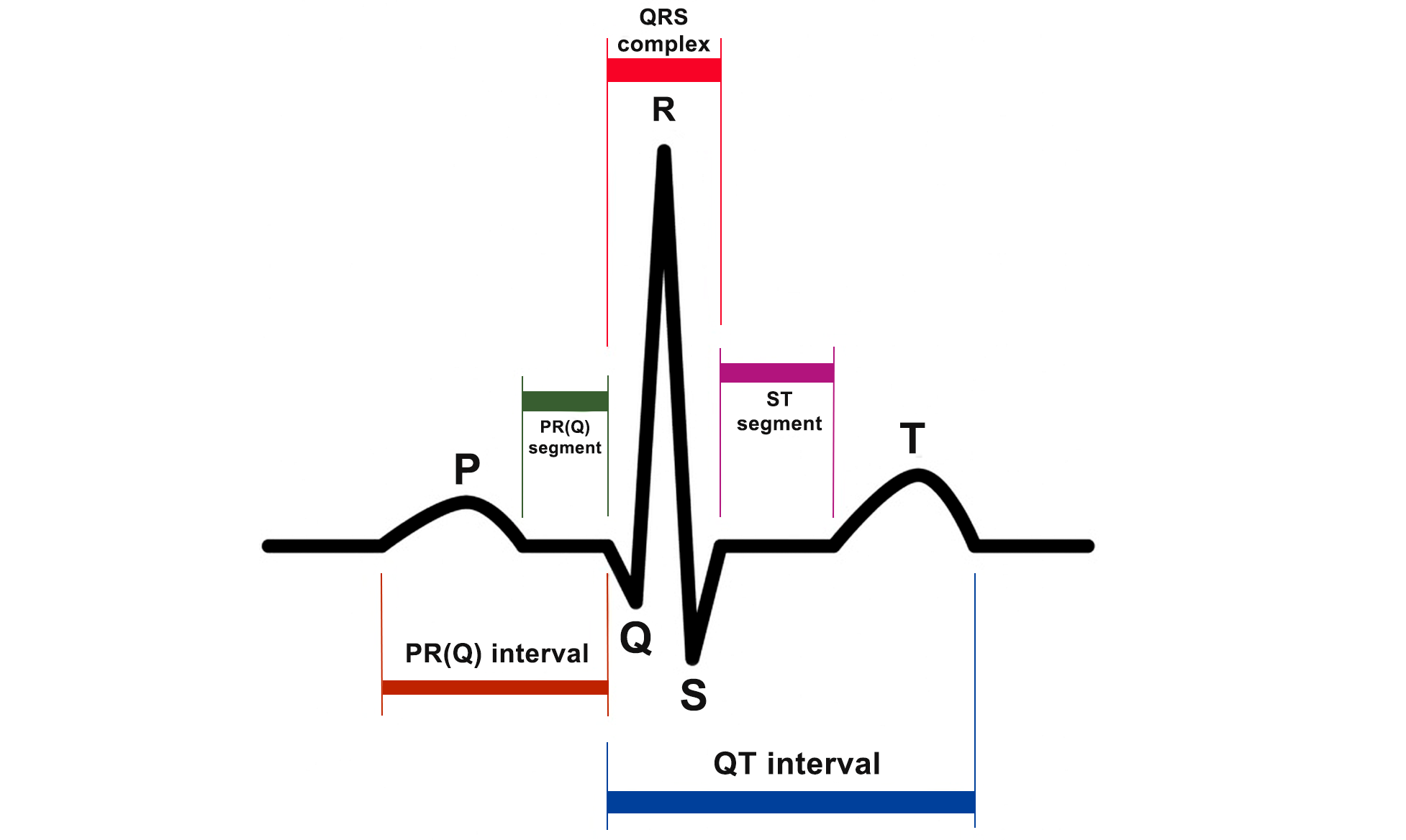
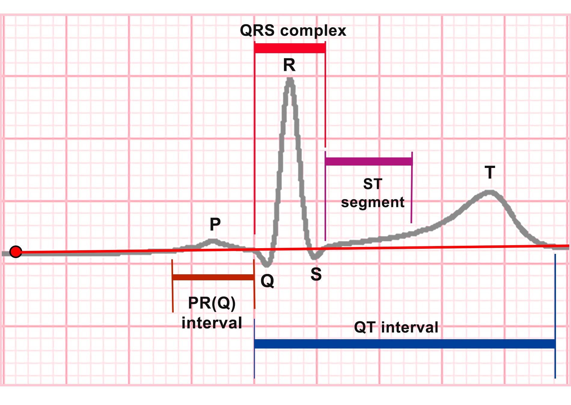
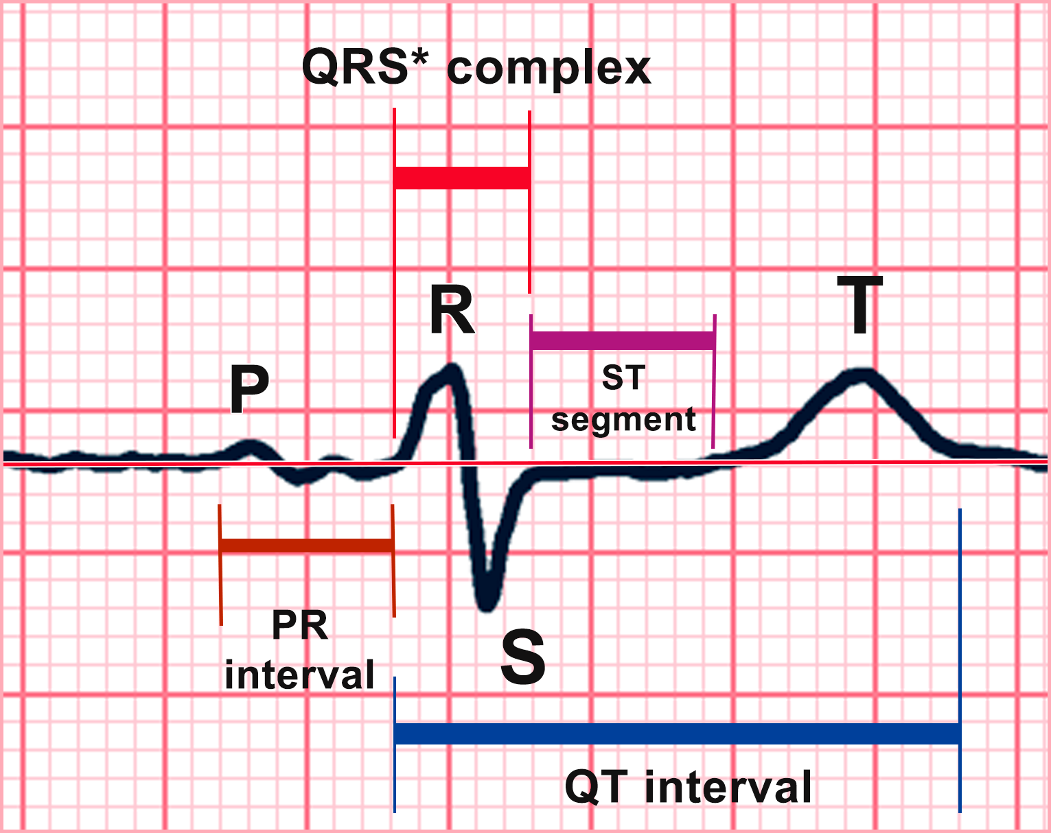
In front of you is a typical, normal ECG complex.

Within it, the main elements can be identified: segments and intervals.

• A segment is the portion between the end of one wave and the beginning of the next.
• An interval is slightly more complex; it is the portion between any two selected points on the ECG tracing.

Looking at this schematic diagram, everything seems clear. However, when analyzing a real ECG recording, questions immediately arise. Therefore, let us see how this looks in real ECG tracings.

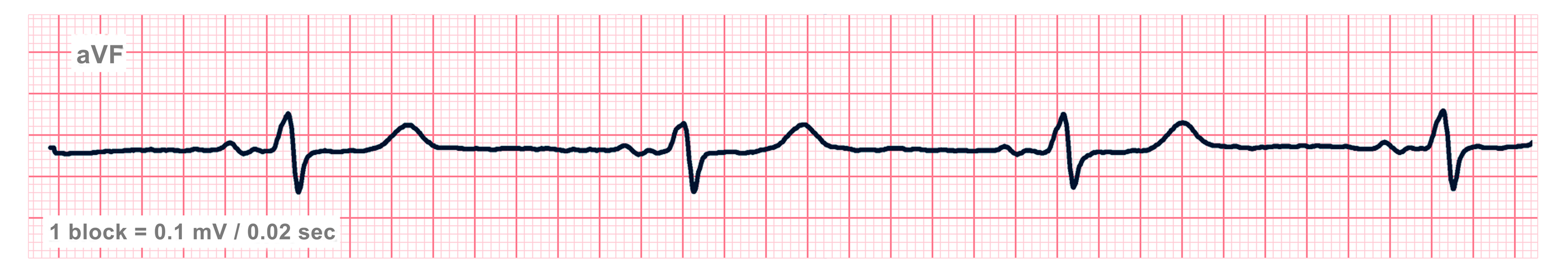
Example 1

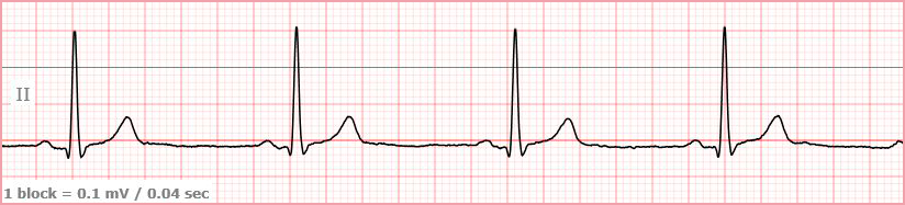
This is a standard complex; it contains all the ECG elements shown in the illustration.

Let us consider another ECG example.

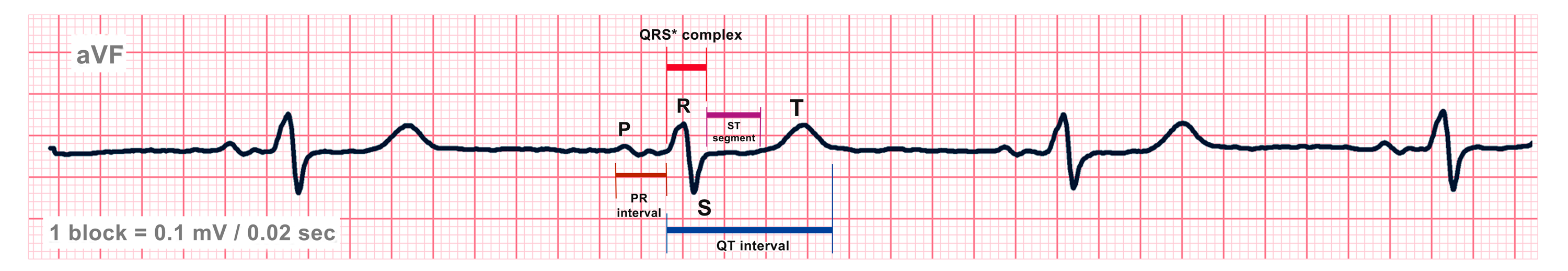
Example 2

Here is an ECG fragment. First, it is necessary to draw the baseline; with experience, you will be able to identify it by eye.

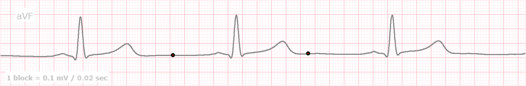
The baseline cannot always be drawn perfectly due to technical artifacts. In this case, we draw it approximately as follows:
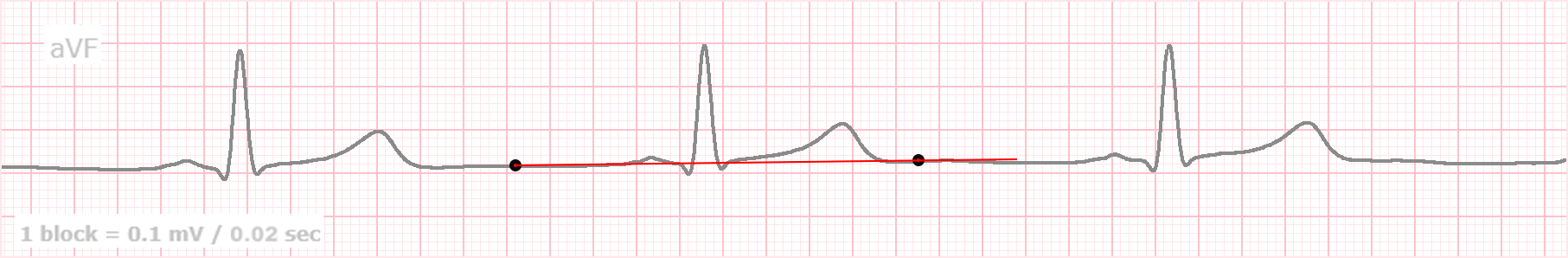And now we identify all those important segments and intervals that we discussed earlier.

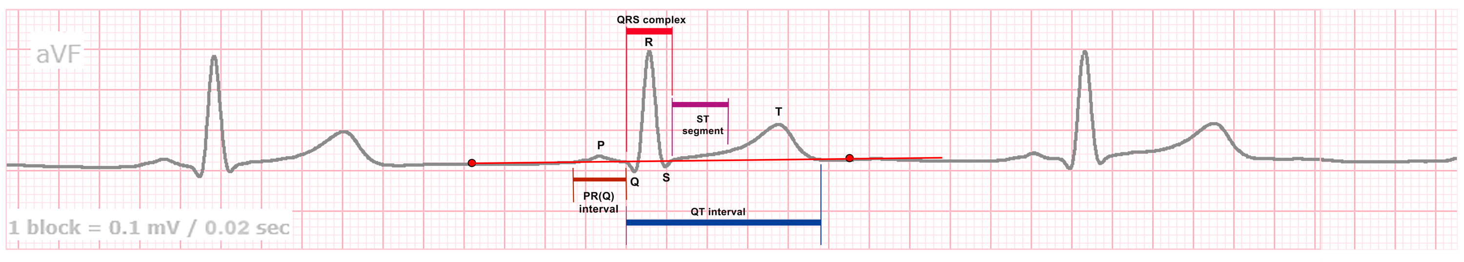
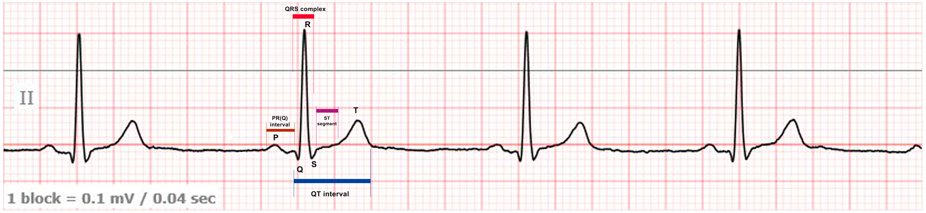
Let us enlarge the image slightly.

This complex is classic; it contains almost all the ECG elements shown in the figure. However, even here some questions remain.

1. Where is the PR (PQ) segment? It is so small that even on the enlarged figure it is difficult to identify clearly. However, it is rarely used in practical analysis, so you do not need to worry about it for now.
2. The ST segment—where is its end? Because it is elevated above the baseline (ST elevation), it is impossible to determine precisely where the T wave begins. One may try to visually extend the T wave toward the baseline, but in practice this is not very important. For ST-segment analysis, only its initial portion is relevant—specifically the first 0.06 s, which on this ECG corresponds to the first 3 mm.
3. Why is the PQ (PR) interval measured from the beginning of the P wave to the beginning of the Q wave, whereas the QT interval is measured from the beginning of Q to the end of T?
   The answer is simple: this convention was established historically—and now we simply have to follow it.

Example 2

Let us identify the segments and intervals that we discussed earlier.

Well, what do you think? Is everything clear here? Or not? The most attentive readers have already noticed some nuances.

Where is the Q wave here? It is absent—we already discussed this in the previous lesson. But then how do we determine the QT interval? It is simple: in this case, we start measuring from the beginning of the R wave. This is not how it appeared in the schematic diagram in the textbook, isn’t it?

But now take a breath and do not worry — this is where the surprises end. We will discuss all of them in detail as you progress through this course.

For now, remember the following: In intervals, we assess their duration (in milliseconds, ms, or seconds), whereas for segments, we are interested only in their position relative to the baseline (above — elevation, below — depression, which is measured in millimeters).

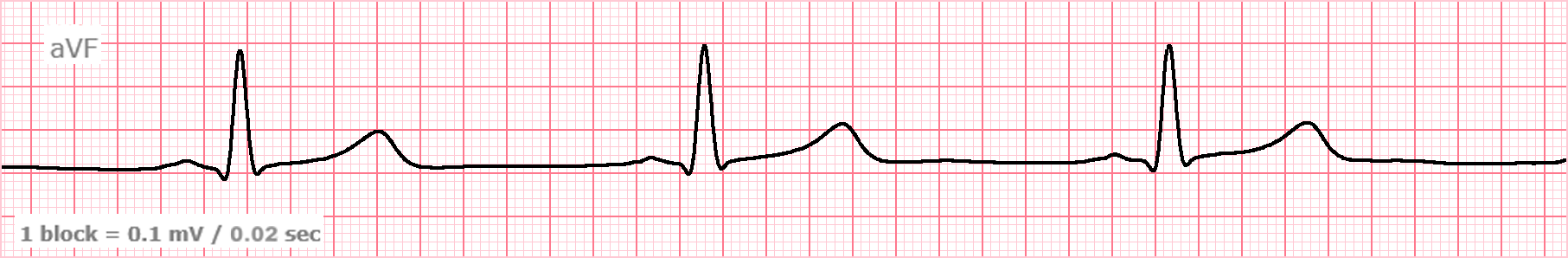
Let us evaluate all the intervals and segments on the last ECG fragment using the markers I have already placed. When you have a paper ECG in front of you, you can simply place a ruler on it, but here you will need to tap the screen a little and strain your eyes.

Note that the paper speed is 25 mm/s, meaning 1 mm corresponds to 0.02 s. 

• The PR interval is 6 mm (small squares). Therefore: PR interval = 6 mm × 0.02 s = 0.12 s, or 120 ms.
• The PR segment is very short and therefore almost impossible to asses
• The QRS* duration, or more precisely the ventricular complex,= 5 mm, therefore:
  5 × 0.02 = 0.10 s, or 100 ms, which is within normal limits.
• As you may remember, for the ST segment, its position relative to the baseline (elevation or depression) is what matters; we will discuss this in more detail soon. In this case, it “lies” on the baseline. The degree of deviation from the baseline, measured in millimeters, is a cornerstone in the diagnosis of ischemia and myocardial infarction.
• The QT interval, in this case measured from the beginning of the R wave, is 20 mm (20 small squares). Therefore: QT interval = 20 × 0.02 = 0.40 s, or 400 ms.

By the way, about the QT interval.

This is a very important interval. Its shortening or prolongation can significantly increase the risk of arrhythmias and sudden cardiac death. Its duration strongly depends on the heart rate (HR): the higher the heart rate, the shorter the QT interval should be, and vice versa. Therefore, for proper evaluation, it is not enough to simply measure it with a ruler. It is also necessary to correct it for heart rate. This corrected value is called QTc.

QTc is calculated using formulas (there are several of them), but we will use the simplest one:

QTc = QT / √RR

Example 3

We determine the duration of the RR and QT intervals.

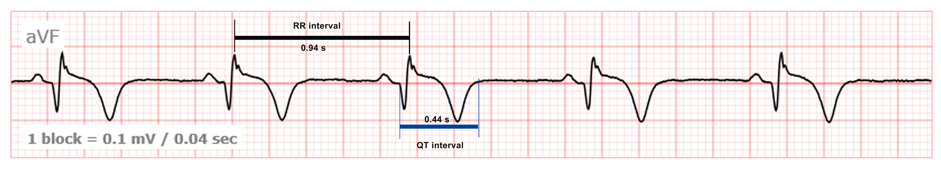
This ECG belongs to a male patient! A QT interval of 0.44 (10×0.04) s is within normal limits, but it requires correction for heart rate. RR 0.94 (23.5 × 0.04). QTc = QT / √RR = 0.44 / √0.94 = 0.453 s, which slightly exceeds the normal limit of 0.45 s.

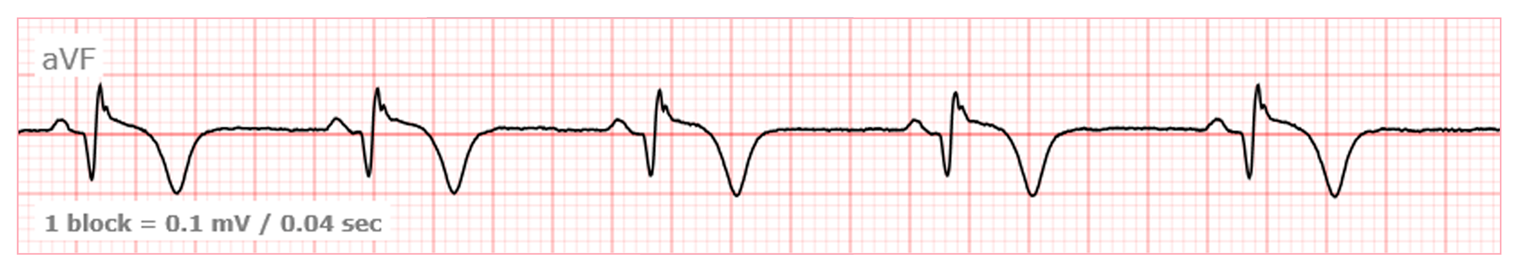
Example 4

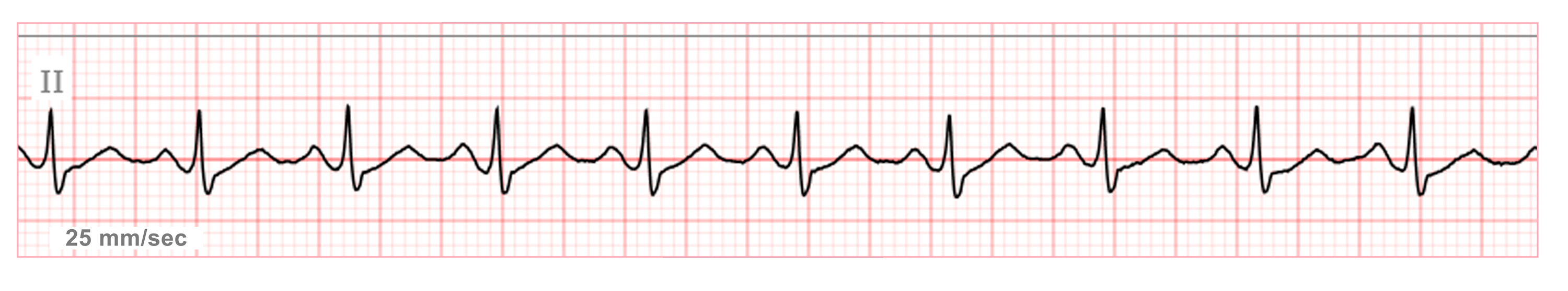
We determine the duration of the RR and QT intervals.
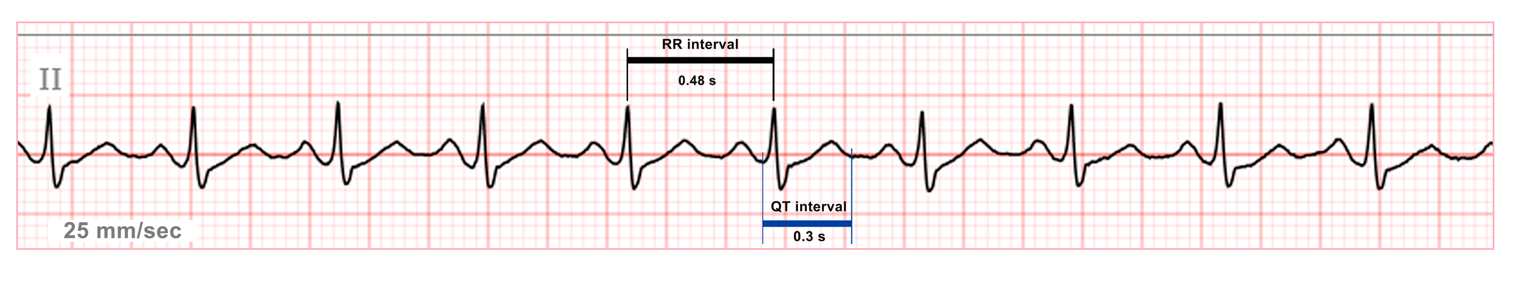The QT interval is 0.3 s (7.5 × 0.04), which is significantly shorter than normal. RR = 0.48 (12 × 0.04) . However, after correction for the heart rate, the QTc turns out to be within normal limits.  QTc = QT / √RR = 0.3 / √0.48 = 0.433 s, which slightly exceeds the normal limit.That is why, when evaluating this interval, one should rely not on the actual QT interval, but on the QTc.

So, the best way to make sense of this “mess” we have created is to complete a self-assessment task. However, the requirements will be strict: I want you to place your “cheat sheet” in front of you and not simply measure the intervals, but also begin interpreting the obtained values. After all, you are a medical professional, not a first-grader seeing a ruler for the first time.